


Time Domain Reflectometer (TDR)
Copyright 1999-2010 Tomi Engdahl
Summary of circuit features
- Brief description of operation: Pulse source for time domain reflecometry
- Circuit protection: Output is short circuit proof
- Circuit complexity: Simple one IC construction, can be built on small piece of veroboard
- Circuit performance: Works very well with cables from 5 meters to 500 meters (no longer cables tested, should work for up to kilometers according the original article)
- Availability of components: Mostly available parts
- This circuit is also available as a kit from Far Circuits
- Design testing: Based on circuit idea published in Electronics Design October 1, 1998 magazine. I built a my own modified version of it which I show in this document. The circuit has been tested with wide variety of cables.
- Applications: Cable cable fault location and transmission line imepdance measurements.
- Extra equipments needed for operation: Oscilloscope needed for making any measurements.
- Power supply: 4.5V battery
- Output pulse amplitude: 4.5 Vpp on untermiated lines, around 2.2Vpp to terminated lines
- Output pulse length: Adjustable from 10 ns to 5 us
- Output impedance: Adjustable from 50 ohm to 100 ohms
- Resolution: Better than 5 ns (around 1 meter of cable)
- Estimated component cost: around 20 dollars including switches, case, knobs
- Safety considerations: The circuit itself works at low voltages and current so it is not dangerous. Making TDR measurements in real life situations can be potentially hazardous on some cases (for example if you accidentally connect equipment to live wire or get lightning induced surge from calbe being measured).
Circuit diagram
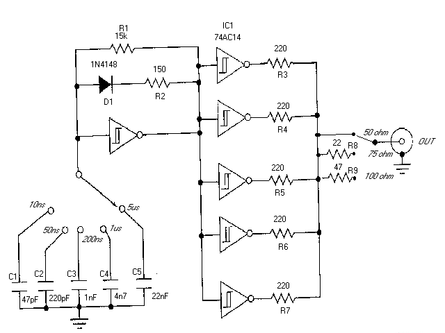
Component list:
R1       15 kohm
R2       150 ohms
R3-R7    220 ohms
R8       22 ohms
R9       47 ohms
C1       47 pF
C2       220 pF
C3       1 nF
C4       4.7 nF
C5       22 nF
D1       1N4148
IC1      74AC14
NOTE: Do not try to substitute IC1 with any other type of IC because the circuit does not well if other 7414 IC type than 74AC14 is used (74HC14 or many other 74xx14 variants do not work well). If you can't find 74AC14 then 74HCT14 could be worth to try, the circuit works with it but with limited performance (impedance matching less accurate, timing not accurate, output pulse shape less optimal). The performance limitations are seen most on the shortest pulse lengths.
Component pinouts
below you can see the pinout if the 74AC14 IC. It is the main IC if the circuit.
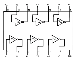
It should not matter which of the ports you use for different parts of the circuit. My recommendation is to use port connected to pins 1 and 2 for the function of the leftmost gate in circuit diagram (the oscillator). Use the rest of the gates for the burering stage (five gates in parallel on the right).
Powering the circuit
This circuit is best powered with 4.5V battery or three 1.5V AA batteries connected in series. The + from battery goes to IC1 pin 14. The pin 7 of IC1 is connected to circuit ground which is connected to circut ground. Remeber to put a 100 nF (ceramic or polypropylene) capacitor between IC1 pins 7 and 14 to guarantee stable operating voltage for the circuit.
Circuit use
TDRs are used in all phases of a cabling system's life, from construction to maintenance and to fault finding. Historically, the TDR has been reserved for only large companies and high level engineers. This was due to the complexity of operation and high cost of the instruments.
If a cable is metal and it has at least two conductors, it can be tested by a TDR. TDRs will troubleshoot and measure all types of twisted pair and coaxial cables. TDRs can locate major or minor cabling problems including; sheath faults, broken conductors, water damage, loose connectors, crimps, cuts, smashed cables, shorted conductors, system components, and a variety of other fault conditions. TDR can be used to locate the problem type and in which place along the calbe the fault is.
The TDR works on the same principle as radar. When that pulse reaches the end of the cable, or a fault along the cable, part or all of the pulse energy is reflected back to the instrument. Any impedance change in cable will cause some energy to reflect back toward the TDR and will be displayed. How much the impedance changes determines the amplitude of the reflection. The TDR measures the time it takes for the signal to travel down the cable, see the problem, and reflect back. The TDR then displays the reflected signal as information on waveform display.
This circuit in this article is made to be used with a normal oscilloscope. The circuit which you build is used as the signal source and the oscilloscope is used as a waveform monitor. Connection diagram:
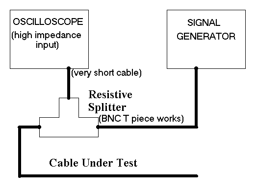
Possible resistive splitter configurations:
                      to oscilloscope
                           |
                           |
                           |
  cable under test --------+--------- signal generator
                      to oscilloscope
                           |
                          | |
                          | | 1 kohm
                          |_|
                           |
  cable under test --------+--------- signal generator
                      to oscilloscope
                           |
                          | |
                          | | 17 ohm
                          |_|
                     ___   |   ___
  cable under test -|___|--+--|___|-- signal generator
                    17 ohm    17 ohm
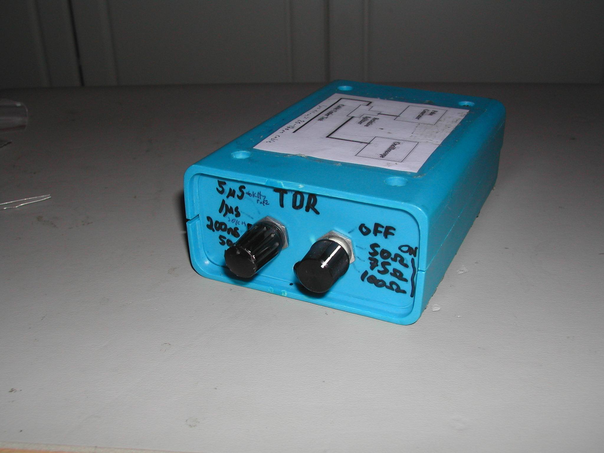
Circuit version with built-in oscilloscope splitter
When using the circuit described eariler I fould out that using external splitter circuit was not convient. I wanted to have a version that had everythign needed in the one package, including some form of trigger output for oscilloscope triggering.
This circuit version that I built has two signal outputs, one for cable to be tested and another for the oscilloscope. This circuit hasl also trigger output for going to oscilloscope trigger input.
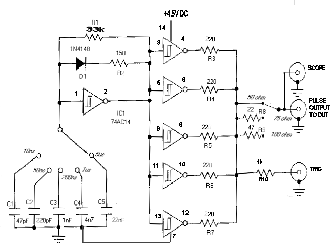
The use of the outputs:
- The PULSE OUTPUT TO DUT goes to the cable being tested.
- The SCOPE output goes directly to the hign impednace oscilloscope signal input using short coaxial cable (I used 15 cm long 50 ohm coaxial cable for this). Do not use a long cable here, because all the cable you add here adds some impedance mismatching to the system (when your cable is lessn than 20 cm the error shiudl not be significant compared to other properties of the circuit)
- The TRIG output goes to the external trigger input on your oscilloscope. Using this cable ans setting your oscilloscope to external trigger mode you get always reliable and accurate scope triggering no matter how mych noise or signal attteuation you see on the line being measured.
Here are some images fo the circuit I built (click images to get bigger view):
Inside of the circuit:
As you can see I have built my circuit to a piece of verboard
(I did not had interrest todesign a special circuit board for this).
The components on the circuit board are wired directly from one
location to another using as short possible leads as possible.
The timing capacitors are all soldered on the back of the
range selection switch. The length of the connection wires
is quite much as short as possible, and the signal wires that
come with ground are wrapped together with their ground wires.
The design does not look nice, but it works well.
This TDR circuit uses very fast signals (over 50 MHz fundametal frequency
and harmonics to well over 100 MHz), so you need to be careful
how you place the component so that the the wires on sensitive
circuit locations are not too long.
Veroboard is not designed for high frequency circuits, but with
careful circuit layout you can use Veroboard successfully even
on high frequency circuits.
Many TDRs have selectable pulse width settings.
The larger the pulse width, the more energy is
transmitted and therefore the further the signal will travel down the cable.
The pulse that the TDR generates takes a certain amount
of time to lauch, and at this time the start of pulse has
already travelled through the cable some distance.
This distance is known as the blind spot. The size of the blind spot varies with the pulse width. The larger the pulse width, the larger the blind spot.
It is difficult to locate a fault contained within the blind spot.
Short pulses are ment to test short cables and to locate faults nearby.
If the fault is very small or cable is very long, the signal strength of a
a very short pulse may not be enough to travel down the cable,
"see" the fault, and travel back. In this case you need to use
longer pulse.
Sometimes, larger pulse widths are helpful even for locating faults that are relatively close. If the fault (impedance mismatch) is very small, the signal strength of a small pulse may not be enough to travel down the cable, .see. the fault, and travel back. The attenuation of the cable combined with the small reflection of a partial fault can make it difficult to detect. A larger pulse width transmits more energy down the cable, making it easier for the TDR to detect a small fault.
This circuit includes settings from 10 nanoseconds to 5 microseconds.
The blind spot for 10 nanosecond pulse is around 4 meters.
With 1 microseconed pulse the blind spot is around 100-130 meters
depending on cable speed.
When you look at the oscilloscope screen you first see the transmitted pulse
and sometime after it you will see the reflected pulse. The second pulse
has the following characteristics on different fault conditions:
TDRs are extremely accurate instruments.
Baslicly the accuracy depends on how accurately you can "read" the pulses on your oscilloscope screen (hoe well they can be "read" and how accurate your oscilloscope timing is). The accuracy does not depends on how accurate components you have used on your pusle signal source.
However, variables in the cable itself can cause errors in distance measurements. When locting distance, you shoul always know correct Velocity of Propagation (VOP) of the cable being tested.
Make a quality connection between the instrument and the cable under test. The importance of a quality connection cannot be overstated. It is best if the cable is adapted to connect directly to the front panel of the instrument. Use adapters, connectors and jumper cables with the same impedance as the cable under test. A poor connection can result in a distorted waveform that can mask a fault.
Remeber to select also right impedance setting from the signal source (the one that matches bet the cable you use).
It is possible to use a TDR to find an approximate value of cable attenuation. Compare the amplitudes of the sent pulse and reflected pulse.
Since the TDR has both the signal source and the receiver located at the same end, the signal will have twice the attenuation because the signal has traveled down and back along the cable. Therefore, if you simply divide the dBRL value by 2, you will have the approximate value of the cable attenuation at that frequency and cable length. Remember, each pulse width has a specific fundamental frequency and cable attenuation is frequency sensitive.
Note the cable length, the pulse width setting, and the return loss of the connections. Make sure the far end of the cable under test is not connected to a terminator or any other piece of equipment.
Structural return loss can be viewed on a TDR by looking at the base line of the waveform. A perfectly flat baseline indicates a high quality cable with no damage or structural return loss. A bumpy baseline would indicate a low-quality cable, damage, and/or structural return loss.
Note: Sometimes DC or low frequency distortion occurs when a pulse is transmitted on a highly capacitive cable such as telephone twisted pair.
Experiment with the TDR on known cable lengths and conditions. Learn to identify waveform signatures and the function of each key. Become familiar with the instrument prior to actual field applications.
A variety of waveforms may be encountered during testing. This variety is due to the different applications, electrical, and environmental characteristic variations found in the cables that exist today.
A complete understanding of the TDR operation and experience in using the instrument is vital to successful use of TDR.
Practice testing on multiple types of known cable segments, with and without components. Become familiar with how each segment looks prior to any problems.
Information on different pulse lengt properties
Tips on making measurements
The signal speed on the cable is typically on a cable is in around
160-240 meter is one microsecond (depends on cable type).
Because the signal you see on oscilloscope
screen has has gone on the way to the fault and back, one microsecond
time in oscilloscope screen is 80-120 meters on typical cables
(usually at 100-110 ,eters per microsecond on normal twisted pair cables).
Pulse length   Fundamental frequency  Blind spot  Approx range (twisted pair)

10 ns            50 MHz                4 m        500 m
50 ns            10 MHz                8 m
200 ns           2.5 MHz               30 m       1.5 km
1 us             500 kHz               100 m      5 km
5 us             100 kHz               600 m
Most information on this tabe are based on technical data given at http://www.riserbond.com/assets/downloads/Appguide.pdf.
Examples of TDR test waveforms
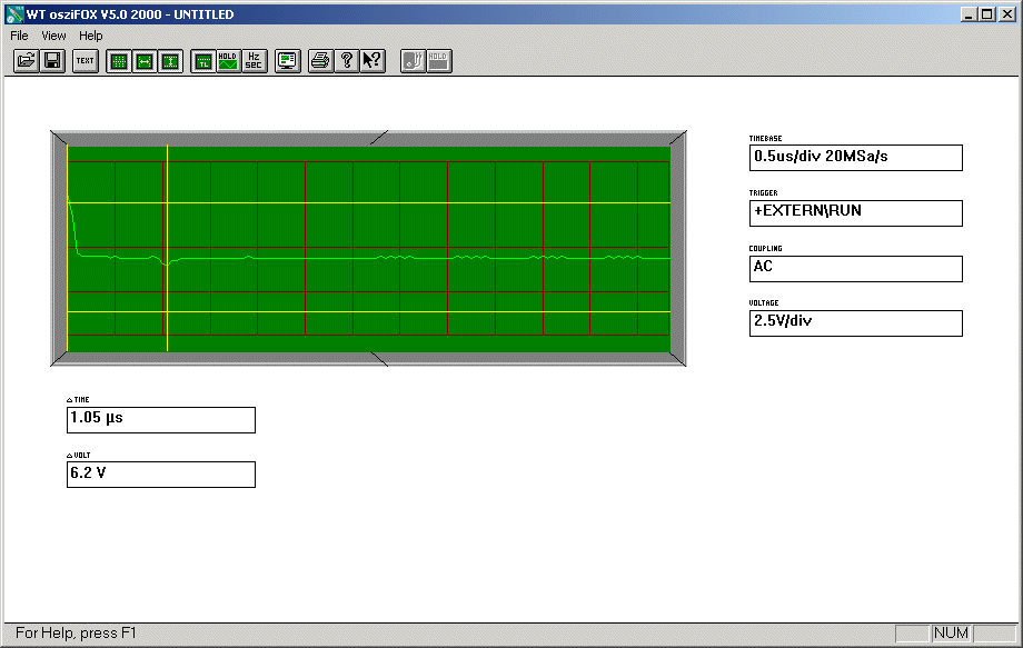
The following tests are performed with 100 meter long CAT5e twisted pair cable. This cable has 100 ohm impedance. One pair of wires is used for testing (wire pair that is connected to RJ-45 connector pins 4 and 5). The signal source is the TDR signal source described at http://www.epanorama.net/circuits/tdr.html. Waveforms are measured with osziFOX handheld oscilloscope. The signals are displayed with 0.5 us/div and 2.5V/div scale. The signals are samples at 20 MSa/s sample rate.
On the left of the oscilloscope picture you see the pulse sent by the TDR signal source. The reflection from the other end of the cable can be seen after it at the location marked with yeallow marker.
Unterminted cable

Short at cable end

Cable terminated with 100 ohm resistor (right termination)

Cable terminated with 50 ohm resistor (wrong impedance termination)
Transmission line theory
If you have learned transmission-line theory during a few lectures in an electromagnetic-fields class, then you learned transmission-line theory with wave equations and a lot of difficult math. Usually it is not much point in trying to work with those equations. With an understanding of the underlying physics, you can often go a lot further in analyzing transmission lines than you can by manipulating dozens of complex equations.
A transmission line is a set of conductors used for transmitting electrical signals. In most discussions of transmission-line theory is the assumption that the lines are uniform.
A uniform transmission line is one whose geometry and materials are uniform. That is, the conductor shape, size, and spacing are constant, and the electrical characteristics of the conductors and the material between them are uniform. Some examples of uniform transmission lines are coaxial cables, twisted-wire pairs, and parallel-wire pairs.
The transmission line, which effectively acts as a transmission medium, guides the signal along the way. The signal travels through this medium at the speed of light within that medium. The speed on the polyethylene insulated RG-59 coaxial cable is for example 66% os the speed of light. For example normal Category 5 cable propagation speed is 66% the speed of light, and for most coaxial cables this value is between 66% and 86%.
You have two models for a transmission line: a circuit comprising infinitesimal inductances and capacitances with parameters L and C and a waveguide for signals with parameters signal speed and characteristic impedance. Although these models are interchangeable, the waveguide model is usually more useful for transmission-line analysis.
Whenever an electromagnetic wave encounters a change in impedance (impedance boundary), some of the signal is transmitted and some of the signal is reflected. The difference between the impedances determines the amplitude of the reflected and transmitted waves. The reflection coefficient, , for the voltage wave is
P=VREFLECTED/VINCIDENT=(Z2-Z1)/(Z2+Z1)
whereas the transmission coefficient is
T=VTRANSMITTED/VINCIDENT =1+p
Amount of reflection is independent of frequency and occurs at all frequencies. You've probably heard or read that transmission-line effects become apparent at higher frequencies, but rarely does anyone explain why. The transmission-line effects (overshoot and oscillation) become apparent when the rise time, tRISE, is short compared with the transmission-line delay, t. When the signal rise time becomes much longer than the transmission-line delay (t), the reflections get "lost" in the transition region. The effect of the reflections then becomes negligible.
A signal traveling along a transmission line has voltage and current waves related by the characteristic impedance of the line. Signal reflections occur at impedance boundaries. As it travels down the line, a signal has delay associated with it.
Transmission-line effects:
- A circuit has reflections unless the transmission-line, source, and load impedances are all equal.
- eflected waves reach the load staggered in time
If we send a pulse (any step function) to a line, this wave travels down the cable and reaches the load at time determined by the cable length and signal speed in the cable. Let's call this time t.
If the cable's characteristic impedance is different from the impedance of the load, some of the incident wave transmits to the load, and some is reflected by the load. The reflected wave travels back through the cable and arrives back at the source at time 2t. If the source impedance does not match the characteristic impedance of the cable, another reflection occurs so that source load absorbs some of the wave, and some is reflected. Subsequent waves arrive at the load in this manner ad infinitum, decreasing in amplitude after each round trip. A simple step signal at the source ends up producing a step wave followed by a series of oscillations at the load (and also seen at source end as well).
Cables used to carry high frequency electrical signals are generally analysed as a form of Transmission Line. The amount of capacitance/metre and inductance/metre depends mainly upon the size and shape of the conductors. The Characteristic Impedance depends upon the ratio of the values of the capacitance per metre and inductance per metre. To understand its meaning, consider a very long run of cable that stretches away towards infinity from a signal source. The result, when the signal power vanishes, never to be seen again, is that the cable behaves like a resistive load of an effective resistance set by the cable itself. This value is called the Characteristic Impedance, of the cable.
Return loss (RL) is a measure of the reflected energy caused by impedance mismatches in the cabling system. Return loss is an important characteristic for any transmission line because it may be responsible for a significant noise component that hinders the ability of the receiver when the data is extracted from the signal. It directly affects "jitter." Return loss is one number which shows cable performance meaning how well it matches the nominal impedance. Poor cable return loss can show cable manufacturing defects and installation defects (cable damaged on installation). With a good quality coaxial cable in good condition you generally get better than -30 dB return loss, and you should generally not got much worse than -20 dB.
Time domain reflectometry theory
Opens, shorts or less-severe impedance discontinuities have a way of showing up on cables in strange places - places you might never suspect. These can occur on coaxial transmission lines or twisted-pair lines. Such opens, shorts or other impedance discontinuities are called faults. The location of faults cannot be determined with simple ohmmeters. Even the existence of certain faults cannot be determined with an ohmmeter. Time domain reflectomer is an instrument often used ot locate such faults. You can use Time Domain Reflectometry to look at the characteristic impedance along the entire length of the cable.
Time Domain Reflectometry measurements (sometimes called Time Domain Spectroscopy techniques) work by injecting a short duration fast rise time pulse into the cable under test. The effect on the cable is measured with an oscilloscope. In a TDR system, a pulse generator injects a fast-rising pulse into a transmission line (usually coaxial cable). The pulse travels the length of the cable, bounces off the far end, and returns through the cable for display on an oscilloscope. Commercial Time Domain Reflectometers incorporate a pulser and scope in a single unit, but in a pinch you can easily put together your own TDR using a pulse generator, scope, and a splitter
The injected pulse radiates down the cable and at the point where the cable ends some portion of the signal pulse is reflected back to the injection point. The amount of the reflected energy is a function of the condition at the end of the cable. In addition to the amount of energy, you can analyze the the reflected signal waveform and timing details to get information on what kind of impedance mismatches can be seen on the cable and where they are located in the cable.
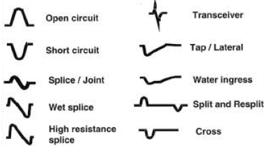
- If the cable is in an open condition the energy pulse reflected back is a significant portion of the injected signal in the same polarity as the injected pulse
- If the other end of the cable is shorted to ground or to the return cable, the energy reflected is in the opposite polarity to the injected signal.
- If the end of the cable is terminated into a resistor with a value matching the characteristic impedance of the cable, all of the injected energy will be absorbed by the terminating resistor and no reflection will be generated.
- If the end of the cable is terminated into a resistor with a value close to cable impedance but not exactly matching the characteristic impedance of the cable, most of the injected energy will be absorbed by the terminating resistor and an a very low amplitude reflection will be generated.
Also any change in the cable impedance due to a connection, major kink or other problem will generate a reflection in addition to the reflection from the end of the cable. By timing the delay between the original pulse and the reflection it is possible to discern the point on the cable length where an anomaly exists. The cable type governs this signal propagation speed, that number can be used to convert the time to cable lehngt. For example normal Category 5 cable propagation speed is 66% the speed of light, and for most coaxial cables this value is between 66% and 86%. Remeber then doing calculations that the time displayed on oscilloscope is twice the cable length, since the signal goes through the cable twice, to the far end and back to the oscilloscope. Commercial TDR units are often calibrated in footage or meters so you don't need to do a conversion from time to distance.
You can get some idea of how severe impedance mismatch happens by looking at the signal amplitude. The more impedance mismatch, more relected energy and thus higher amplitude reflected signal. Usually it is hard to make any accurate judgements on the reflected signal amplitude, because typically the cable attenuation causes lots of signal attenuation. So more far away the impedance mismatch is, the weaker the signal gets before you see it. If you know the cable attenuation characteristics or have some value to compare the signal amplitude (some other known impedance mismatch on same cable nearby what you are measuring), then you might try to make some educated quess how severe the problem is. When thinking of the signal attenuation on the cable, please note that since the signal goes through the cable twice, to the far end and back to the oscilloscope, you need to count the cable attenuation twice.
Two types of stimulus pulses are commonly used for TDR; impulse, and step-voltage.
- Impulse type TDR is somewhat crude, brute-force method useful mainly for cable length measurements and for locating gross fault conditions like a severed cable, a dead short, or a really bad kink.
- The step-voltage system allows measurent of the impedance of the cable, any connectors or splices, and the termination at the end. (The step pulse needs to be at least twice as long as the cable's delay time.)
The TDR circuit presented in this article is designed for impulse type measurements in mind. This is easier and adequate for many uses. The waveforms generatred by impulse type signal source are easier to "read".
The circuit can be used also for step-voltage system measurements by selecting the longest pulse lenght that the circuit generates and use the start of that pulse as the step signal.
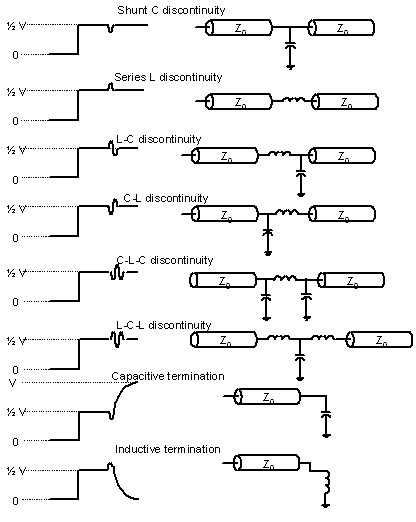
The TDR waveform shows the effect of all the reflections created by all of the impedance discontinuities. The waveform is like a road map of the impedance variations across the transmission line. The waveform can be evaluated to determine how much the impedance deviates from the nominal value.
Different TDR systems have different performacne characteristics. Several factors affect a TDR system's ability to resolve closely-spaced discontinuities. If a TDR system has insufficient resolution, small or closely-spaced discontinuities may be smoothed together into a single aberration in the waveform. This effect may not only obscure some discontinuities, but it also may lead to inaccurate impedance readings.
Rise time, settling time and pulse aberrations of the stimulus can also significantly affect a TDR system's resolution. Two neighboring discontinuities may be indistinguishable to the measurement instrument if the distance between them amounts to less than half the system rise time. While in many cases the fastest rise time available is desirable, very fast rise times can, in some cases, give misleading results on a TDR measurement. Aberrations that occur prior to the main incident step can be particularly troublesome because they arrive at a discontinuity and begin generating reflections before the main step arrives. These early reflections reduce resolution by obscuring closely-spaced discontinuities. Aberrations, such as ringing, that occur after the incident step will cause corresponding aberrations in the reflections. These aberrations will be difficult to distinguish from the reflections caused by discontinuities in the device-under-test (DUT).
Many factors contribute to the accuracy of a TDR measurement. These include the TDR system.s step response, interconnect reflections and DUT losses, step amplitude accuracy, baseline correction and the accuracy of the reference impedance (ZO) used in the measurements. All TDR measurements are relative; they are made by comparing reflected amplitudes to an incident amplitude.
Random noise can be a significant source of error when making measurements of small impedance variations.
Cable losses in the test setup can cause several problems. While both conductor loss and dielectric loss can occur, conductor loss usually dominates. Conductor loss is caused by the finite resistance of the metal conductors in the cable which, due to the skin effect, increases with frequency. The result of this incremental series resistance is an apparent increase in impedance as you look further into the cable. So, with long test cables, the DUT impedance looks higher than it actually is. The second problem is that the rise time and settling of the incident pulse is degraded by the time it reaches the end of the cable. This affects resolution and accuracy since the effective amplitude of the incident step is different than expected.
Looking at the TDR signals
You need a fast oscilloscope to get nice measurement results from the TDR measurements. Generally the faster the better. I have made some basic measurements with 20 MHz analogue oscilloscope and 20 megasamples per second digital samplign oscilloscope (osziFox). With such equipment, the measurement accuracy is limited to few meters at the best. You can get information if something is terribly wrong and where is the problem. And you can measure length of long cables (tens of meters with accuracy of few meters). But using such oscilloscpe will not show you all the fine details of the wiring.
If you have access to oscilloscope with 100 MHz or 1 GHz sample rate, you can get much more accurate measurements.
Here ase some example waveforms you can see on oscilloscope screen and that kind of wiring problems can cause them:
Here are some waveforms that different electronics components and circuits cause:
NOTE: When using an expensive high bandwidth oscilloscope, you need to be very careful with it. High-bandwidth sampling heads are often extremely static-sensitive. To ensure their continued performance in impedance and signal integrity applications, they require protection devices above and beyond those which suffice for conventional oscilloscopes. You should cap sampling inputs when not in use, use grounded wrist straps when workign with device and always discharge the device being measured before probing or connecting it to the module (touching the probe ground lead to the point you want to TDR test). It is a good idea to connect DUT cable wires to ground before making any measurements. In case your oscilloscope is a high frequency scope with 50 ohm input impedance, I recommend to consider using 1 kohm resistive probe for making measurements.
Differential TDR Measurements
Nowadays many high-speed designs are implemented with differential transmission lines. Differential transmission lines are used for example to carry Ethernet signals (UTP cable) and also to carry telecom signals (PSTN, ADSL, T1 etc..).
All of the single-ended TDR measurement concepts discussed so far also apply to differential transmission lines. However, they must be extended to provide useful measurements of differential impedance.
A differential transmission line has two unique modes of propagation, each with its own characteristic impedance and propagation velocity. Much of the literature refers to these as the odd mode and the even mode.
- The odd mode impedance is defined as the impedance measured by observing one line, while the other line is driven by a complementary signal.
- The differential impedance is the impedance measured across the two lines with the pair driven differentially. Differential impedance is twice the odd mode impedance.
- The even mode impedance is defined as the impedance measured by observing one line, while the other line is driven by an equivalent signal as the first.
- The common mode impedance is the impedance of the lines connected together in parallel, which is half the even mode impedance.
Tying together the two conductors in a differential line and driving them with a traditional single-ended TDR system, will yield a good measure of common mode impedance.
To provide true differential impedance measurements, you would need a signal source that can give two polarity-selectable TDR step for each of two channels. With this approach, the differential system can actually be driven differentially. You need also differential input module for oscilloscope to measure the differential signals on the cable. True differential TDR measurements require that both the stimulus and the acquisition systems be well matched in terms of timing and step response. Poor matching between the cables or interconnect devices and the DUT will skew the TDR steps in time when they arrive at the DUT, even if they are aligned at the instrument.s front panel, causing significant measurement error.
Need for TDR measurements
Signal integrity is an issue that grows more important with each |successive advancement in system clock and data rates. A key predictor for signal integrity is the impedance of the environment. cables, connectors, package leads, and circuit board traces - through which signals must travel. Consequently, impedance measurements have become part of almost every high-speed design project.
Time Domain Reflectometry is a convenient, powerful tool for characterizing impedance of single-ended and differential transmission lines and networks. A TDR instrument takes advantage of the fact that any change in impedance in a transmission line or network causes reflections that are a function of magnitude of the discontinuity.
Time Domain Reflectometry is used nowadays in both electronics laboratories to test electronics circuit and connection systems performance. Time Domain Reflectometry is also used in many fields where testing of different cabling systems are needed. This technology is used to test the quality of wiring used in structured cabling systems and for looking shorts / open circuits on cabling systems. Different kinds of TDR instruments are used by telephone company periar persons, cable TV repair persons and repair crews of power companies. Time domain reflectometry (TDR) was originally developed by the power and communications industries to locate faults and breaks in cables.
Time domain reflectometry (TDR) is a also used in geotechnical field instrumentation as a method of locating the depth to a shear plane or zone in a landslide. TDR uses an electronic voltage pulse that is reflected like radar from a damaged location in a coaxial cable. To monitor slope movement, coaxial cables are grouted in boreholes and interrogated using a cable tester. Characteristic cable signatures can be stored and compared over time for changes, indicating slope movement. For example RG59/U cable manufactured by Belden (www.belden.com) and other manufacturers is inexpensive and easy to use for this kind of applications, but for best best results jacketed, foam-filled cable is recommended at http://www.iti.northwestern.edu/publications/tdr/kane/msmwtdr.pdf. TDR technology is also used on some soil moisture measurements as well.
There are modern commercial TDR-capable instruments that can automatically compare the incident and reflected amplitudes to provide a direct readout of impedance, reflection coefficient and time for both common mode and differential impedance. In addition, some of them have waveform math functions built into the instrument to automatically display TDR results for a user-selected rise time. There are also TDR instruments designed for fiber optic networks measurements (those are called OTDR). There are several types of TDR baed cable testers on the market, targeted for different application fields like electronics laboratories, cable measurements on the field and for soil measurements.
Related information:
- Tomi's blog postings related to TDR
- TDR circuit modification idea
- TDR Circuit kit
- TDR Circuit kit details
Information sources:
- Build Your own Cable Radar, Electronics Design magazine October 1, 1998, pages 97-98 (web version at http://www.elecdesign.com/Articles/ArticleID/6260/6260.html)
- http://www.edn.com/article/CA56702.html
- Introduction to Metallic Time Domain Reflectometry
- Transmission line measurements at ePanorama.net
- TDR Impedance Measurements: A Foundation for Signal Integrity
- Monitoring Slope Movement with Time Domain Reflectometry
More information
Good sites to look for further information how to use a TDR:
Tomi Engdahl <[email protected]>